Bỏ qua nội dung chính

Làm thế nào để tìm thứ sáu đầu tiên hoặc cuối cùng của mỗi tháng trong Excel?

Thông thường thứ sáu là ngày làm việc cuối cùng trong tháng. Làm thế nào bạn có thể tìm thấy thứ sáu đầu tiên hoặc cuối cùng dựa trên một ngày nhất định trong Excel? Trong bài viết này, chúng tôi sẽ hướng dẫn bạn cách sử dụng hai công thức để tìm ngày thứ sáu đầu tiên hoặc cuối cùng của mỗi tháng.

Tìm thứ sáu đầu tiên của một tháng
Tìm thứ sáu cuối cùng của tháng


Tìm thứ sáu đầu tiên của một tháng

Ví dụ: có một ngày nhất định 1/1/2015 nằm trong ô A2 như ảnh chụp màn hình bên dưới. Nếu bạn muốn tìm thứ sáu đầu tiên của tháng dựa trên ngày đã cho, vui lòng thực hiện như sau.

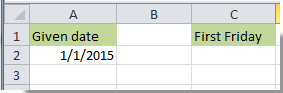
1. Chọn một ô để hiển thị kết quả. Ở đây chúng tôi chọn ô C2.

2. Sao chép và dán công thức dưới đây vào nó, sau đó nhấn đăng ký hạng mục thi Chìa khóa.

=CEILING(EOMONTH(A2,-1)-5,7)+6

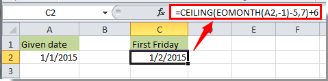
Sau đó, ngày được hiển thị trong ô C2, có nghĩa là ngày thứ sáu đầu tiên của tháng 2015 năm 1 là ngày 2/2015/XNUMX.

Chú ý:

1. Nếu bạn muốn tìm ngày thứ sáu đầu tiên của các tháng khác, vui lòng nhập ngày được chỉ định của tháng đó vào ô A2, rồi sử dụng công thức.

2. Trong công thức, A2 là ô tham chiếu mà ngày đã cho định vị. Bạn có thể thay đổi nó để đáp ứng nhu cầu của bạn.

Tìm thứ sáu cuối cùng của tháng

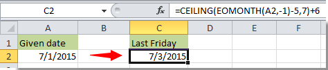
Ngày đã cho 1/1/2015 nằm trong ô A2, để tìm ngày thứ sáu cuối cùng của tháng này trong Excel, vui lòng thực hiện như sau.

1. Chọn một ô, sao chép công thức bên dưới vào đó, sau đó nhấn đăng ký hạng mục thi phím để nhận kết quả.

=DATE(YEAR(A2),MONTH(A2)+1,0)+MOD(-WEEKDAY(DATE(YEAR(A2),MONTH(A2)+1,0),2)-2,-7)

Sau đó, thứ sáu cuối cùng của tháng 2015 năm 2 sẽ hiển thị ô BXNUMX.

Chú thích: Bạn có thể thay đổi A2 trong công thức thành ô tham chiếu của ngày đã cho của bạn.


Các bài liên quan:

Công cụ năng suất văn phòng tốt nhất

🤖 Trợ lý AI của Kutools: Cách mạng hóa việc phân tích dữ liệu dựa trên: Thực thi thông minh   |  Tạo mã  |  Tạo công thức tùy chỉnh  |  Phân tích dữ liệu và tạo biểu đồ  |  Gọi các hàm Kutools...
Các tính năng phổ biến: Tìm, đánh dấu hoặc xác định các bản sao   |  Xóa hàng trống   |  Kết hợp các cột hoặc ô mà không làm mất dữ liệu   |   Vòng không có công thức hữu ích. Cảm ơn !
Siêu tra cứu: Nhiều tiêu chí VLookup    VLookup Nhiều Giá Trị  |   VLookup trên nhiều trang tính   |   Tra cứu mờ ....
Danh sách thả xuống nâng cao: Tạo nhanh danh sách thả xuống   |  Danh sách thả xuống phụ thuộc   |  Danh sách thả xuống nhiều lựa chọn ....
Trình quản lý cột: Thêm một số cột cụ thể  |  Di chuyển cột  |  Chuyển đổi trạng thái hiển thị của các cột ẩn  |  So sánh dãy và cột hữu ích. Cảm ơn !
Các tính năng nổi bật: Tiêu điểm lưới   |  Chế độ xem thiết kế   |   Thanh công thức lớn    Trình quản lý sổ làm việc & trang tính   |  Thư viện tài nguyên (Văn bản tự động)   |  Bảng chọn ngày   |  Kết hợp các bảng tính   |  Mã hóa/Giải mã ô    Gửi email theo danh sách   |  Siêu lọc   |   Bộ lọc đặc biệt (lọc in đậm/nghiêng/gạch ngang...) ...
15 bộ công cụ hàng đầu12 bản văn CÔNG CỤ (thêm văn bản, Xóa ký tự,...)   |   50 + Biểu đồ Các loại (Biểu đồ Gantt,...)   |   40+ Thực tế Công thức (Tính tuổi dựa trên ngày sinh,...)   |   19 chèn CÔNG CỤ (Chèn mã QR, Chèn ảnh từ đường dẫn,...)   |   12 Chuyển đổi CÔNG CỤ (Số thành từ, Chuyển đổi tiền tệ,...)   |   7 Hợp nhất & Tách CÔNG CỤ (Các hàng kết hợp nâng cao, Chia ô,...)   |   ... và nhiều hơn nữa

Nâng cao kỹ năng Excel của bạn với Kutools for Excel và trải nghiệm hiệu quả hơn bao giờ hết. Kutools for Excel cung cấp hơn 300 tính năng nâng cao để tăng năng suất và tiết kiệm thời gian.  Bấm vào đây để có được tính năng bạn cần nhất...

Mô tả


Tab Office mang lại giao diện Tab cho Office và giúp công việc của bạn trở nên dễ dàng hơn nhiều

  • Cho phép chỉnh sửa và đọc theo thẻ trong Word, Excel, PowerPoint, Publisher, Access, Visio và Project.
  • Mở và tạo nhiều tài liệu trong các tab mới của cùng một cửa sổ, thay vì trong các cửa sổ mới.
  • Tăng 50% năng suất của bạn và giảm hàng trăm cú nhấp chuột cho bạn mỗi ngày!
Comments (12)
Rated 5 out of 5 · 1 ratings
This comment was minimized by the moderator on the site
Even shorter 😅
=lambda(Date;WeekDay;EOMONTH(Date;0)-WEEKDAY(EOMONTH(Date;0);WeekDay+10)+1
Where "WeekDay" parameter is 1=Monday, 7=Sunday
This comment was minimized by the moderator on the site
=lambda(Date;WeekDay;EOMONTH(Date;0)-WEEKDAY(EOMONTH(Date;0);WeekDay+10)+1)

I forgot a bracket at the end
This comment was minimized by the moderator on the site
Vậy công thức tính thứ sáu tuần thứ 2 của tháng như thế nào vậy ban?
This comment was minimized by the moderator on the site
Hi Tâm Cao Điền,
Suppose you want to calculate the second friday of the month based on the given date in A1, you can try the following formula:
=A18-DAY(A18)+CHOOSE(WEEKDAY(A18-DAY(A18),2),11,10,9,8,14,13,12)
This comment was minimized by the moderator on the site
porque cuando lo pruebo tal cual me sale error ?
o sea estoy copiando y pegando y no funciona

alguien sabe?
This comment was minimized by the moderator on the site
Hi andre,
Can you tell me which formula you used in the post? And what error your are experiencing?
This comment was minimized by the moderator on the site
Why not make the "last Friday" formula: =CEILING(EOMONTH(A2,0)-5,7)-1? That works for all dates I have tried....
This comment was minimized by the moderator on the site
Hi Eric,
I hop you are still on this forum and receive my reply.
Thanks so much for an EASY formula. I've never encountered =CEILING.
Rated 5 out of 5
This comment was minimized by the moderator on the site
Hi Eric,
Thanks for sharing it.
This comment was minimized by the moderator on the site
Hello and thank you for this formula. I am not an Excel guru and acnnot easily work out how to change this formula for the last Friday to be the Last Monday, or any other day. Can you please explain how to interpret this.
This comment was minimized by the moderator on the site
Matt,

The way the formula works is: First we find the last day of the month with the EOMONTH() function. For the last day of the current month, we use "0" as the month offset. For the previous month, it would be -1. (Either "=EOMONTH(A2,0)" or "=EOMONTH(A2,-1)".)

Then, in the "=CEILING()" function, we subtract the number of days required to bring us back to Sunday from the day for which we are searching. (For Tuesday, it would be -2, so we make the formula so far: "=CEILING(EOMONTH(A2,0)-2...."

We use the "significance" value of "7" because weeks are seven days long (of course).This finds the date of either the previous Saturday, or the following Saturday (Excel dates started with 1/1/1900, which was a Sunday. So if you enter a "1" in cell A2 with the Long Date format, the cell would read: "Sunday, January 1, 1900".). For that reason, the =CEILING() function, using "7" as the "significance" argument returns Saturday, which is always a multiple of 7 in Excel. Now the formula is "=CEILING(EOMONTH(A2,0)-2,7...".

Now we need to return the date to a Tuesday, so we either subtract 4 for the last Tuesday of the month, or add 3 for the first Tuesday of the next month. So the final formula is, respectively, either "=CEILING(EOMONTH(A2,0)-2,7)-4" or "=CEILING(EOMONTH(A2,0)-2,7)+3".

We can work through the math by assuming the last day of the month is either a Monday (assume its value is 9 - for ease of illustration, so the values do not go negative) or a Wednesday (assume value 11). "EOMONTH()" will return either of those days (9 or 11). Subtracting 2 results in the previous Saturday (value 7) or Monday (value 9), respectively. The CEILING() function then returns, respectively, the previous Saturday (value 7, because the ceiling of 7 with significance 7 is 7) or the current Saturday (value 14, because the ceiling of 9, significance 7, is 14). Subtracting 4 results in the previous Tuesday (value 3) or the current week's Tuesday (value 10), respectively. For the first Tuesday of the following month, adding 3 to the Saturday value (7 or 14) returns either Tuesday value 10, or Tuesday value 17, respectively.


Hopefully that helps you understand so that you can modify the formula as necessary. You can even change it to find the second Tuesday, or second to last Tuesday, by adding or subtracting an additional 7, respectively.
This comment was minimized by the moderator on the site
Hi Matt,
You just need to change the last number -7 to -1 to solove the problem.
=DATE(YEAR(A2),MONTH(A2)+1,0)+MOD(-WEEKDAY(DATE(YEAR(A2),MONTH(A2)+1,0),2)-2,-1)
There are no comments posted here yet
Please leave your comments in English
Posting as Guest
×
Rate this post:
0   Characters
Suggested Locations