Bỏ qua nội dung chính

Làm cách nào để trả về nhiều giá trị phù hợp dựa trên một hoặc nhiều tiêu chí trong Excel?

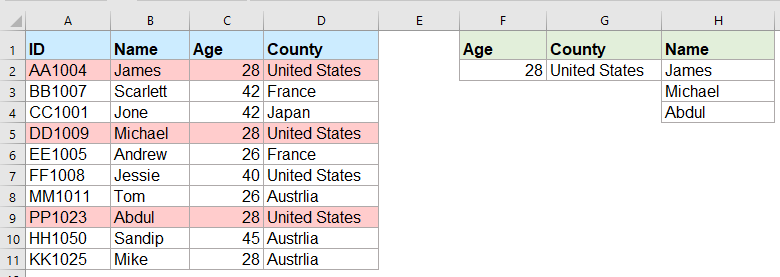
Thông thường, hầu hết chúng ta đều dễ dàng tra cứu một giá trị cụ thể và trả về mục phù hợp bằng cách sử dụng hàm VLOOKUP. Tuy nhiên, bạn đã bao giờ cố gắng trả về nhiều giá trị phù hợp dựa trên một hoặc nhiều tiêu chí như ảnh chụp màn hình sau đây chưa? Trong bài viết này, tôi sẽ giới thiệu một số công thức để giải quyết công việc phức tạp này trong Excel.

Trả về nhiều giá trị phù hợp dựa trên một hoặc nhiều tiêu chí với công thức mảng


Trả về nhiều giá trị phù hợp dựa trên một hoặc nhiều tiêu chí với công thức mảng

Ví dụ: tôi muốn trích xuất tất cả các tên có tuổi 28 và đến từ Hoa Kỳ, vui lòng áp dụng công thức sau:

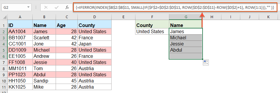
1. Sao chép hoặc nhập công thức dưới đây vào một ô trống mà bạn muốn xác định kết quả:

=INDEX($B$2:$B$11, SMALL(IF(COUNTIF($F$2, $C$2:$C$11)*COUNTIF($G$2, $D$2:$D$11), ROW($A$2:$D$11)-MIN(ROW($A$2:$D$11))+1), ROW(A1)), COLUMN(A1))

Chú thích: Trong công thức trên, B2: B11 là cột mà giá trị khớp được trả về từ đó; F2, C2: C11 là điều kiện đầu tiên và dữ liệu cột chứa điều kiện đầu tiên; G2, D2: D11 là điều kiện thứ hai và dữ liệu cột chứa điều kiện này, vui lòng thay đổi chúng theo nhu cầu của bạn.

2. Sau đó nhấn Ctrl + Shift + Enter để nhận kết quả phù hợp đầu tiên, sau đó chọn ô công thức đầu tiên và kéo chốt điền xuống các ô cho đến khi giá trị lỗi được hiển thị, bây giờ, tất cả các giá trị phù hợp được trả về như hình minh họa bên dưới:

Lời khuyên: Nếu bạn chỉ cần trả về tất cả các giá trị phù hợp dựa trên một điều kiện, vui lòng áp dụng công thức mảng bên dưới:

=IFERROR(INDEX($B$2:$B$11, SMALL(IF($F$2=$D$2:$D$11, ROW($D$2:$D$11)-ROW($D$2)+1), ROW(1:1))),"" )


Các bài viết tương đối hơn:

  • Trả lại nhiều giá trị tra cứu trong một ô được phân tách bằng dấu phẩy
  • Trong Excel, chúng ta có thể áp dụng hàm Vlookup để trả về giá trị phù hợp đầu tiên từ một ô trong bảng, nhưng đôi khi, chúng ta cần trích xuất tất cả các giá trị phù hợp và sau đó được phân tách bằng dấu phân cách cụ thể, chẳng hạn như dấu phẩy, dấu gạch ngang, v.v. thành một ô như ảnh chụp màn hình sau được hiển thị. Làm cách nào chúng ta có thể lấy và trả về nhiều giá trị tra cứu trong một ô được phân tách bằng dấu phẩy trong Excel?
  • Vlookup và trả lại nhiều giá trị phù hợp cùng một lúc trong Google Trang tính
  • Chức năng Vlookup thông thường trong Google sheet có thể giúp bạn tìm và trả về giá trị khớp đầu tiên dựa trên một dữ liệu nhất định. Tuy nhiên, đôi khi, bạn có thể cần vlookup và trả về tất cả các giá trị phù hợp như hình minh họa sau. Bạn có cách nào hay và dễ dàng để giải quyết công việc này trong Google sheet không?
  • Vlookup và trả lại nhiều giá trị từ danh sách thả xuống
  • Trong Excel, làm thế nào bạn có thể vlookup và trả về nhiều giá trị tương ứng từ danh sách thả xuống, có nghĩa là khi bạn chọn một mục từ danh sách thả xuống, tất cả các giá trị tương đối của nó được hiển thị cùng một lúc như ảnh chụp màn hình sau. Bài viết này, tôi sẽ giới thiệu giải pháp từng bước.
  • Vlookup và trả về nhiều giá trị theo chiều dọc trong Excel
  • Thông thường, bạn có thể sử dụng hàm Vlookup để nhận giá trị tương ứng đầu tiên, nhưng đôi khi, bạn muốn trả về tất cả các bản ghi phù hợp dựa trên một tiêu chí cụ thể. Bài viết này, tôi sẽ nói về cách vlookup và trả về tất cả các giá trị phù hợp theo chiều dọc, chiều ngang hoặc vào một ô duy nhất.
  • Vlookup và trả về dữ liệu khớp giữa hai giá trị trong Excel
  • Trong Excel, chúng ta có thể áp dụng hàm Vlookup thông thường để nhận giá trị tương ứng dựa trên một dữ liệu nhất định. Tuy nhiên, đôi khi, chúng tôi muốn vlookup và trả về giá trị khớp giữa hai giá trị như ảnh chụp màn hình sau được hiển thị, làm thế nào bạn có thể giải quyết tác vụ này trong Excel?


  • Thanh siêu công thức (dễ dàng chỉnh sửa nhiều dòng văn bản và công thức); Bố cục đọc (dễ dàng đọc và chỉnh sửa số lượng ô lớn); Dán vào Dải ô đã Lọchữu ích. Cảm ơn !
  • Hợp nhất các ô / hàng / cột và Lưu giữ dữ liệu; Nội dung phân chia ô; Kết hợp các hàng trùng lặp và Tổng / Trung bình... Ngăn chặn các ô trùng lặp; So sánh các dãyhữu ích. Cảm ơn !
  • Chọn trùng lặp hoặc duy nhất Hàng; Chọn hàng trống (tất cả các ô đều trống); Tìm siêu và Tìm mờ trong Nhiều Sổ làm việc; Chọn ngẫu nhiên ...
  • Bản sao chính xác Nhiều ô mà không thay đổi tham chiếu công thức; Tự động tạo tài liệu tham khảo sang Nhiều Trang tính; Chèn Bullets, Hộp kiểm và hơn thế nữa ...
  • Yêu thích và Chèn công thức nhanh chóng, Dãy, Biểu đồ và Hình ảnh; Mã hóa ô với mật khẩu; Tạo danh sách gửi thư và gửi email ...
  • Trích xuất văn bản, Thêm Văn bản, Xóa theo Vị trí, Xóa không gian; Tạo và In Tổng số phân trang; Chuyển đổi giữa nội dung ô và nhận xéthữu ích. Cảm ơn !
  • Siêu lọc (lưu và áp dụng các lược đồ lọc cho các trang tính khác); Sắp xếp nâng cao theo tháng / tuần / ngày, tần suất và hơn thế nữa; Bộ lọc đặc biệt bằng cách in đậm, in nghiêng ...
  • Kết hợp Workbook và WorkSheets; Hợp nhất các bảng dựa trên các cột chính; Chia dữ liệu thành nhiều trang tính; Chuyển đổi hàng loạt xls, xlsx và PDFhữu ích. Cảm ơn !
  • Nhóm bảng tổng hợp theo số tuần, ngày trong tuần và hơn thế nữa ... Hiển thị các ô đã mở khóa, đã khóa bởi các màu sắc khác nhau; Đánh dấu các ô có công thức / tênhữu ích. Cảm ơn !
tab kte 201905
  • Cho phép chỉnh sửa và đọc theo thẻ trong Word, Excel, PowerPoint, Publisher, Access, Visio và Project.
  • Mở và tạo nhiều tài liệu trong các tab mới của cùng một cửa sổ, thay vì trong các cửa sổ mới.
  • Tăng 50% năng suất của bạn và giảm hàng trăm cú nhấp chuột cho bạn mỗi ngày!
officetab dưới cùng


Comments (25)
No ratings yet. Be the first to rate!
This comment was minimized by the moderator on the site
Hi, if there are duplicate values (e.g. two adams), how do i make sure that it only returns 1 adam and not 2?
This comment was minimized by the moderator on the site
Hello, Bobby,
To extract only unique matching values, you should apply the below formula:
After pasting the formula, please press Ctrl + Shift + Enter keys together to get the correct result.
=IFERROR(INDEX($B$2:$B$5, MATCH(0, COUNTIF(H1:$H$1, $B$2:$B$5)+IF($D$2:$D$5<>$G$2, 1, 0)+IF($C$2:$C$5<>$F$2, 1, 0), 0)), "")

Please have a try, hope it can help you!
This comment was minimized by the moderator on the site
Hi,

Thanks for posting these examples.
I'm trying to implement this in my own sheet, but don't get it to work (maybe because I'm using an europe version of excel)?

I want to get the dates of the days that I had my shifts or that I have worked 'some' (>0) hours for a client.

So in I3 is the name and in J3 the month. K3 and L3 are the shifts (1 is worked) and hours (don't know how to set this, should be more than zero)

My expected results are in:
Shifts: I7 and I8
hours: J7

So I worked more than 0 hours for 'person 2' in oktober on 3-10-2022
had shifts for person 2 on '10-10-2022' and 28-10-2022

When I add '=INDEX($B$2:$B$11, SMALL(IF(COUNTIF($F$2, $C$2:$C$11)*COUNTIF($G$2, $D$2:$D$11), ROW($A$2:$D$11)-MIN(ROW($A$2:$D$11))+1), ROW(A1)), COLUMN(A1))' in my excel sheet, it doesn't allow the comma between the different parts of the formula.
So I need to change them to ';'.
But when I try it it always says: '#NAME?'

So can someone help me with this?

Kind regards,

Bas
[img]https://drive.google.com/file/d/1iIPQKuj_PNhqWyWlwJ4IQTqGNEd6B9Hw/view?usp=share_link[/img]
This comment was minimized by the moderator on the site
Hi,

First, thank you for sharing!

Can you please provide a solution to the case below:

I have 3 columns (A: Containing reference information, B: Containing information to be searched, C: Search result)

Image url is provided below

https://ibb.co/VHCd09K

Column A-------------------------Column B------------Column C
File Name-------------------------Name----------------File Name, Document Name, Element Name, Name
Changed Element-----------------Element--------------Changed Element, Element Name, Element ID
Column Location
Document Name
Element Name
Name
Category
Warranty
Slope
Element ID

What I need is to search in column A for any partial match with cell B2 (Name) or B3 (Element) and get the result in one cell,

Thank you, Behzad
This comment was minimized by the moderator on the site
Hello, Behzad
Maybe the below User Defined Function can help you.
Public Function ConcatPartLookUp(rngInput As Range, rngSource As Range, Optional strDelimiter As String, Optional blCaseSensitive)
Dim rng As Range
If strDelimiter = "" Then strDelimiter = ","
If IsMissing(blCaseSensitive) Then
    blCaseSensitive = False
Else
    blCaseSensitive = True
End If
For Each rng In rngSource
    If blCaseSensitive Then
        If InStr(1, rng.Value, rngInput.Value, vbBinaryCompare) > 0 Then ConcatPartLookUp = ConcatPartLookUp & strDelimiter & rng.Value
    Else
        If InStr(1, rng.Value, rngInput.Value, vbTextCompare) > 0 Then ConcatPartLookUp = ConcatPartLookUp & strDelimiter & rng.Value
    End If
Next
If Len(ConcatPartLookUp) > 0 Then ConcatPartLookUp = Mid(ConcatPartLookUp, 2, Len(ConcatPartLookUp))
End Function


After copying and pasting this code, and then use this formula:=ConcatPartLookUp(B2,$A$2:$A$8) to get the result you need.
Please have a try, hope it can help you!
This comment was minimized by the moderator on the site
Heyi, thank you for the formula. It worked for "fixed" values / text as criterias. However, one of the criterias i'm trying to use is a condition (values <>0 ), but does not work the described formula. Do you guys know what should i change to adapt the formula so I can have a condition as one of the criterias, please?

Best,

João
This comment was minimized by the moderator on the site
Hello, Marcus
To solve your problem, please view this article:
https://www.extendoffice.com/documents/excel/6393-excel-vlookup-function.html#b3-2
There are some detailed explanations of this task. You just need to change the criteira to your own.
Thank you!
This comment was minimized by the moderator on the site
Hi,

if in cell H1 i write "Name" and wanted to link that with the formula, how would that work?
Then I could write "ID" in cell H1 and would automatically get as a result: AA1004; DD1009; PP1023 (for the first formula)

Thank you in advance!
This comment was minimized by the moderator on the site
Hello, Marie
Sorry, i can't get the point of your first problem, could you explain your problem more clearly and detailedly? Or you can insert a screenshot here to describe your problem.
As for the second question, you just need to change the cell reference as this:
=INDEX($A$2:$A$11, SMALL(IF(COUNTIF($F$2, $C$2:$C$11)*COUNTIF($G$2, $D$2:$D$11), ROW($A$2:$D$11)-MIN(ROW($A$2:$D$11))+1), ROW(A1)), COLUMN(A1))

Remeber to press Ctrl + Shift + Enter keys together.
Please try, hope it can help you!
This comment was minimized by the moderator on the site
Hello,
what would be needed to expand the first formula in the following case:
Some IDs are Blank (e.g. cell A5 is blank) and I would like an additional condition outputting lines only when the IDs are not blank. (So the output should then be James and Abdul.
Thanks!
This comment was minimized by the moderator on the site
Hello, Jo,
To solve your problem, please apply the below formula:
=INDEX($B$2:$B$11, SMALL(IF(COUNTIF($F$2, $C$2:$C$11)*COUNTIF($G$2, $D$2:$D$11)*($A$2:$A$11<>0), ROW($A$2:$D$11)-MIN(ROW($A$2:$D$11))+1), ROW(A1)), COLUMN(A1))

Please have a ry, hope it can help you!
This comment was minimized by the moderator on the site
hello,
ive tried using the formula and it either generates a value of 0 or the image attached
This comment was minimized by the moderator on the site
Hello, Milku
Your screenshot showed WPS software of MAC version, so I am not sure whether our formula is available.
I uploaded an Excel file to here, you can try to see if it can calculate correctly in you environment.
Thank you!
This comment was minimized by the moderator on the site
When I use the second formula and drag down, nothing appears. The formula result (fx) says it should be returning something but it is blank. How do I correct this?
This comment was minimized by the moderator on the site
Hello Alysia,

Glad to help. I tried the second formula in the article and drag the formula down, the rest of results were returned. I think there may be two reasons for your problem. First, maybe you forget to press Ctrl + Shift + Enter keys to enter the formula. Second, the matching result is only one, so no other results are not returned. Please have a check.

Sincerely,
Mandy
This comment was minimized by the moderator on the site
Hi,

I was wondering if it at all possible to enter a 2nd criteria but from the same range as the 1st criteria,

For example with the used example above i would like to search for the names of people from both America and France So cell F3 would have France, Scarlett & Andrew would also populate in the list in Column G

Thank you for assistance in advance.
This comment was minimized by the moderator on the site
Hello Nick,

Glad to help. If you want to get the names of people from both America and France, I advise you to use our formula twice to get the result. Please see the screenshot, In F2 and G2 are values "United States" and "France". Apply formula =IFERROR(INDEX($B$2:$B$11, SMALL(IF($F$2=$D$2:$D$11, ROW($D$2:$D$11)-ROW($D$2)+1), ROW(1:1))),"" ) to get the results for America. And apply formula =IFERROR(INDEX($B$2:$B$11, SMALL(IF($G$2=$D$2:$D$11, ROW($D$2:$D$11)-ROW($D$2)+1), ROW(1:1))),"" ) to get the results for France. It's simple. Please have a try.

Sincerely,
Mandy
This comment was minimized by the moderator on the site
In the first example, what change to the formula would be needed to return everyone who was less than 28 years old?
There are no comments posted here yet
Load More
Please leave your comments in English
Posting as Guest
×
Rate this post:
0   Characters
Suggested Locations