Bỏ qua nội dung chính

Làm thế nào để hiển thị tên tương ứng của điểm cao nhất trong Excel?

Tác giả: Tiểu Dương Sửa đổi lần cuối: 2020-11-20

Giả sử, tôi có dải dữ liệu gồm hai cột - cột tên và cột điểm tương ứng, bây giờ, tôi muốn lấy tên của người đạt điểm cao nhất. Có cách nào tốt để giải quyết vấn đề này một cách nhanh chóng trong Excel không?

Hiển thị tên tương ứng của điểm cao nhất với các công thức


mũi tên màu xanh bong bóng bên phải Hiển thị tên tương ứng của điểm cao nhất với các công thức

Để truy xuất tên của người đạt điểm cao nhất, các công thức sau đây có thể giúp bạn lấy kết quả.

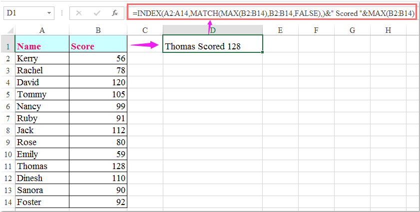
Vui lòng nhập công thức này: =INDEX(A2:A14,MATCH(MAX(B2:B14),B2:B14,FALSE),)&" Scored "&MAX(B2:B14) vào một ô trống nơi bạn muốn hiển thị tên, rồi nhấn đăng ký hạng mục thi phím để trả về kết quả như sau:

doc hiển thị tên điểm cao nhất 1

Ghi chú:

1. Trong công thức trên, A2: A14 là danh sách tên mà bạn muốn lấy tên từ đó và B2: B14 là danh sách điểm.

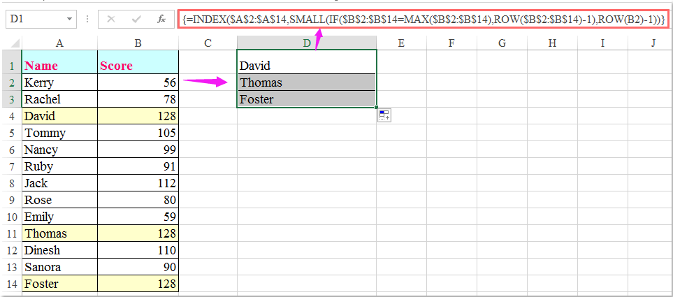
2. Công thức trên chỉ có thể lấy tên nếu có nhiều hơn một tên có cùng điểm cao nhất, để lấy tất cả các tên có điểm cao nhất, công thức mảng sau đây có thể giúp bạn.

Nhập công thức này:

=INDEX($A$2:$A$14,SMALL(IF($B$2:$B$14=MAX($B$2:$B$14),ROW($B$2:$B$14)-1),ROW(B2)-1)), và sau đó nhấn Ctrl + Shift + Enter các phím với nhau để hiển thị tên, sau đó chọn ô công thức và kéo chốt điền xuống cho đến khi giá trị lỗi xuất hiện, tất cả các tên có điểm cao nhất được hiển thị như ảnh chụp màn hình bên dưới:

doc hiển thị tên điểm cao nhất 2

Công cụ năng suất văn phòng tốt nhất

🤖 Trợ lý AI của Kutools: Cách mạng hóa việc phân tích dữ liệu dựa trên: Thực thi thông minh   |  Tạo mã  |  Tạo công thức tùy chỉnh  |  Phân tích dữ liệu và tạo biểu đồ  |  Gọi các hàm Kutools...
Các tính năng phổ biến: Tìm, đánh dấu hoặc xác định các bản sao   |  Xóa hàng trống   |  Kết hợp các cột hoặc ô mà không làm mất dữ liệu   |   Vòng không có công thức hữu ích. Cảm ơn !
Siêu tra cứu: Nhiều tiêu chí VLookup    VLookup Nhiều Giá Trị  |   VLookup trên nhiều trang tính   |   Tra cứu mờ ....
Danh sách thả xuống nâng cao: Tạo nhanh danh sách thả xuống   |  Danh sách thả xuống phụ thuộc   |  Danh sách thả xuống nhiều lựa chọn ....
Trình quản lý cột: Thêm một số cột cụ thể  |  Di chuyển cột  |  Chuyển đổi trạng thái hiển thị của các cột ẩn  |  So sánh dãy và cột hữu ích. Cảm ơn !
Các tính năng nổi bật: Tiêu điểm lưới   |  Chế độ xem thiết kế   |   Thanh công thức lớn    Trình quản lý sổ làm việc & trang tính   |  Thư viện tài nguyên (Văn bản tự động)   |  Bảng chọn ngày   |  Kết hợp các bảng tính   |  Mã hóa/Giải mã ô    Gửi email theo danh sách   |  Siêu lọc   |   Bộ lọc đặc biệt (lọc in đậm/nghiêng/gạch ngang...) ...
15 bộ công cụ hàng đầu12 bản văn CÔNG CỤ (thêm văn bản, Xóa ký tự,...)   |   50 + Biểu đồ Các loại (Biểu đồ Gantt,...)   |   40+ Thực tế Công thức (Tính tuổi dựa trên ngày sinh,...)   |   19 chèn CÔNG CỤ (Chèn mã QR, Chèn ảnh từ đường dẫn,...)   |   12 Chuyển đổi CÔNG CỤ (Số thành từ, Chuyển đổi tiền tệ,...)   |   7 Hợp nhất & Tách CÔNG CỤ (Các hàng kết hợp nâng cao, Chia ô,...)   |   ... và nhiều hơn nữa

Nâng cao kỹ năng Excel của bạn với Kutools for Excel và trải nghiệm hiệu quả hơn bao giờ hết. Kutools for Excel cung cấp hơn 300 tính năng nâng cao để tăng năng suất và tiết kiệm thời gian.  Bấm vào đây để có được tính năng bạn cần nhất...

Mô tả


Tab Office mang lại giao diện Tab cho Office và giúp công việc của bạn trở nên dễ dàng hơn nhiều

  • Cho phép chỉnh sửa và đọc theo thẻ trong Word, Excel, PowerPoint, Publisher, Access, Visio và Project.
  • Mở và tạo nhiều tài liệu trong các tab mới của cùng một cửa sổ, thay vì trong các cửa sổ mới.
  • Tăng 50% năng suất của bạn và giảm hàng trăm cú nhấp chuột cho bạn mỗi ngày!
Comments (17)
No ratings yet. Be the first to rate!
This comment was minimized by the moderator on the site
Hi sir, I tried this method, But the problem is if top two students have the same score when I look for the highest 3 one student's name alone is repeated twice with the same score instead of second student's name. How to solve this.
This comment was minimized by the moderator on the site
Hello, Divyanathan
Maybe the following array formula can help you:

=IFERROR(INDEX(A:A,SUM(IF(($B$2:$B$100+ROUND(0.1/ROW($B$2:$B$100),5))=LARGE($B$2:$B$100+ROUND(0.1/ROW($B$2:$B$100),5),ROW(A1)),ROW($B$2:$B$100)))),"")


Note: After inserting the formula, please press Ctrl + Shift + Enter keys together to get the first result, and then drga this formula cell down to get the largest n results as you need.

Please have a try, hope it can help you!
This comment was minimized by the moderator on the site
Hola disculpa me podrías apoyar para sacar la formula o otro tipo de dato que me pueda dar el nombre del tota de un resultado?

explico tengo una tabla con 4 nombres diferentes distribuidos en las celdas C3,D3,E3 y F3 de las cuales cada celda mencionada tiene rangos de productos ejemplo: detergentes
y cada celda mencionada tiene precios diferentes.
en el resultado que debo de mostrar es el valor mínimo de precio de cada detergente de las celdas ya mencionadas arriba, y a lo que quiero llegar es que indique una formula o un dato que indique que en cada resultado a la derecho me indique el nombre del valor de resultado.
muestro un ejemplo mas especifico: en la celda <C3> tiene un nombre de insumos, en la celda C4 hasta C120 están los precios de cada detergente que maneja la celda C3, en la celda <D3> esta un nombre de biodetergentes, y mismo proceso la celda D4 hasta D120 están los precios en la celda G4 se encuentra el resultado del valor mínimo de estos dos nombres (insumos-biodetergentes) teniendo el valor menor el de nombre de insumos. ahora en la celda H4 quiero que me aparezca el nombre del valor de resultado en este caso que me aparezca el nombre de "insumos" como puedo hacer para que me aparezca este nombre? espero me allá podido dar a entender de lo que requiero
muchas gracias por su atención
saludos cordiales.
This comment was minimized by the moderator on the site
ik heb het ook geprobeerd met alle dezelfde gegevens zoals in het voorbeeld maar het werkt totaal niet
This comment was minimized by the moderator on the site
Hello jac, Sorry to hear that. As I have answered in the below comment, the two formulas work great for me. And I have been wondering why the formulas aren't working for the readers. There are two reasons that can lead to the malfunction of the second formula. 
First, if you are using Excel versions before Excel 2020, then you must enter the formula =INDEX($A$2:$A$14,SMALL(IF($B$2:$B$14=MAX($B$2:$B$14),ROW($B$2:$B$14)-1),ROW(B2)-1)) via pressing Ctrl + Shift + Enter keys together.
Second, When you get the first result, remember to select the formula cell and drag the fill handle down until error value appears. So all the other results will be returned.
And as you can see in the screenshots below, the two formulas are working fine for me.  Hope my solution works. Have a nice day.
Sincerely,Mandy
This comment was minimized by the moderator on the site
bullshitdoes not work
This comment was minimized by the moderator on the site
Hello,
Sorry to hear that. But I did tried the two formulas in the article and both of them works perfectly. Please see the screenshots I uploaded here. And we would love to solve the problem for you if you can provide the details of the problem. Looking forward to your reply.Sincerely,Mandy
This comment was minimized by the moderator on the site
Trying to do the same thing but with the minimum score in Microsoft sheets. I swapped max for min as below and it didn't work =INDEX($A$2:$A$14,SMALL(IF($B$2:$B$14=MIN($B$2:$B$14),ROW($B$2:$B$14)-1),ROW(B2)-1))
This comment was minimized by the moderator on the site
Hi. This formula was exactly what I was looking for. However is there a way do this with the lowest Score but above 0 (in my case £00.00) I removed the bit of formula that displays the amount as only needed the Name and comment.I changed the MAX for MIN but there are a few entries at 0 (£00.00) and formula displays the name for the first of the '0' entries
This comment was minimized by the moderator on the site
Hello, Nigel,To lookup the lowest value above 0, you should apply the below array formula:After entering the formula, please remember to press Ctrl + Shift + Enter keys together to get the correct result.=INDEX(A2:A8,MATCH(MIN(IF(B2:B8>0,B2:B8)),B2:B8,0))&" Scored "&MIN(IF(B2:B8>0,B2:B8))
Please try, hope it can help you!
This comment was minimized by the moderator on the site
How do you find the second highest student? Please help me :( I only get the name of Thomas.
This comment was minimized by the moderator on the site
How do you find the second highest student?
This comment was minimized by the moderator on the site
How would you show two names if the high scores match?
This comment was minimized by the moderator on the site
Hello, Chris,
To get all names if there are multiple high scores match, the second formula in this article can do you a favor.
Please try it, thank you!
This comment was minimized by the moderator on the site
How would you get the matching numbers with the corresponding names to display horizontally?
There are no comments posted here yet
Load More
Please leave your comments in English
Posting as Guest
×
Rate this post:
0   Characters
Suggested Locations