Bỏ qua nội dung chính

Làm thế nào để tính tổng dựa trên tiêu chí cột và hàng trong Excel? 

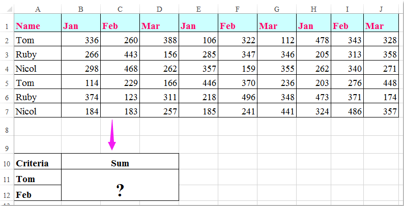
Tôi có một dải dữ liệu chứa tiêu đề hàng và cột, bây giờ, tôi muốn lấy tổng các ô đáp ứng cả tiêu chí tiêu đề cột và tiêu đề hàng. Ví dụ, để tính tổng các ô mà tiêu chí cột là Tom và tiêu chí hàng là tháng hai như sau được hiển thị ảnh chụp màn hình. Bài viết này, tôi sẽ nói về một số công thức hữu ích để giải quyết nó.

doc sum cột hàng tiêu chí 1

Tính tổng các ô dựa trên tiêu chí cột và hàng với các công thức


mũi tên màu xanh bong bóng bên phải Tính tổng các ô dựa trên tiêu chí cột và hàng với các công thức

Tại đây, bạn có thể áp dụng các công thức sau để tính tổng các ô dựa trên cả tiêu chí cột và hàng, vui lòng thực hiện như sau:

Nhập bất kỳ công thức nào dưới đây vào ô trống mà bạn muốn xuất kết quả:

=SUMPRODUCT((A2:A7="Tom")*(B1:J1="Feb")*(B2:J7))

=SUM(IF(B1:J1="Feb",IF(A2:A7="Tom",B2:J7)))

Và sau đó nhấn Shift + Ctrl + Nhập các phím với nhau để lấy kết quả, xem ảnh chụp màn hình:

doc sum cột hàng tiêu chí 2

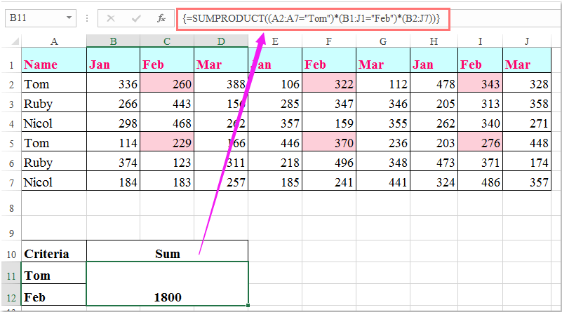
Chú thích: Trong các công thức trên: TomTháng Hai là tiêu chí cột và hàng dựa trên, A2: A7, B1: J1 tiêu đề cột và tiêu đề hàng có chứa tiêu chí không, B2: J7 là phạm vi dữ liệu mà bạn muốn tính tổng.

Công cụ năng suất văn phòng tốt nhất

🤖 Trợ lý AI của Kutools: Cách mạng hóa việc phân tích dữ liệu dựa trên: Thực thi thông minh   |  Tạo mã  |  Tạo công thức tùy chỉnh  |  Phân tích dữ liệu và tạo biểu đồ  |  Gọi các hàm Kutools...
Các tính năng phổ biến: Tìm, đánh dấu hoặc xác định các bản sao   |  Xóa hàng trống   |  Kết hợp các cột hoặc ô mà không làm mất dữ liệu   |   Vòng không có công thức hữu ích. Cảm ơn !
Siêu tra cứu: Nhiều tiêu chí VLookup    VLookup Nhiều Giá Trị  |   VLookup trên nhiều trang tính   |   Tra cứu mờ ....
Danh sách thả xuống nâng cao: Tạo nhanh danh sách thả xuống   |  Danh sách thả xuống phụ thuộc   |  Danh sách thả xuống nhiều lựa chọn ....
Trình quản lý cột: Thêm một số cột cụ thể  |  Di chuyển cột  |  Chuyển đổi trạng thái hiển thị của các cột ẩn  |  So sánh dãy và cột hữu ích. Cảm ơn !
Các tính năng nổi bật: Tiêu điểm lưới   |  Chế độ xem thiết kế   |   Thanh công thức lớn    Trình quản lý sổ làm việc & trang tính   |  Thư viện tài nguyên (Văn bản tự động)   |  Bảng chọn ngày   |  Kết hợp các bảng tính   |  Mã hóa/Giải mã ô    Gửi email theo danh sách   |  Siêu lọc   |   Bộ lọc đặc biệt (lọc in đậm/nghiêng/gạch ngang...) ...
15 bộ công cụ hàng đầu12 bản văn CÔNG CỤ (thêm văn bản, Xóa ký tự,...)   |   50 + Biểu đồ Các loại (Biểu đồ Gantt,...)   |   40+ Thực tế Công thức (Tính tuổi dựa trên ngày sinh,...)   |   19 chèn CÔNG CỤ (Chèn mã QR, Chèn ảnh từ đường dẫn,...)   |   12 Chuyển đổi CÔNG CỤ (Số thành từ, Chuyển đổi tiền tệ,...)   |   7 Hợp nhất & Tách CÔNG CỤ (Các hàng kết hợp nâng cao, Chia ô,...)   |   ... và nhiều hơn nữa

Nâng cao kỹ năng Excel của bạn với Kutools for Excel và trải nghiệm hiệu quả hơn bao giờ hết. Kutools for Excel cung cấp hơn 300 tính năng nâng cao để tăng năng suất và tiết kiệm thời gian.  Bấm vào đây để có được tính năng bạn cần nhất...

Mô tả


Tab Office mang lại giao diện Tab cho Office và giúp công việc của bạn trở nên dễ dàng hơn nhiều

  • Cho phép chỉnh sửa và đọc theo thẻ trong Word, Excel, PowerPoint, Publisher, Access, Visio và Project.
  • Mở và tạo nhiều tài liệu trong các tab mới của cùng một cửa sổ, thay vì trong các cửa sổ mới.
  • Tăng 50% năng suất của bạn và giảm hàng trăm cú nhấp chuột cho bạn mỗi ngày!
Comments (17)
No ratings yet. Be the first to rate!
This comment was minimized by the moderator on the site
Brilliant!

The function =SUM(IF(B1:J1="Feb",IF(A2:A7="Tom",B2:J7))) is a great X & Y summation tool.
I would not have thought this logic out on my own.
In fact i took me a minute to deconstruction the operations.

Thank you
This comment was minimized by the moderator on the site
My data that I am trying to retrieve is in a table. Would this impact the result at all? I have:

=SUM(IF('[Primary Controller Active Project Database (KC notes)1.xlsx]Active Project Tracking'!$B2:$B66=X2,IF('[Primary Controller Active Project Database (KC notes)1.xlsx]Active Project Tracking'!$A1:$AV1=AH10,'[Primary Controller Active Project Database (KC notes)1.xlsx]Active Project Tracking'!$H$2:$AV$66)))

So I think the equivalent would be if you did your information above, but in a table in a different workbook. Thoughts?
This comment was minimized by the moderator on the site
If there were negatives in the matrix and you only wanted to include the positives, what would you do? 
I tried to do something like this:

=SUMPRODUCT((Column = Criteria)* ( Row = Criteria) * (second column = Criteria) * (Matrix) * (Matrix >0))

This comment was minimized by the moderator on the site
Is there a way to do this but instead of writing "Tom" & "Feb" in the formula, you are able to reference the criteria cells e.g.A11 & A12?
This comment was minimized by the moderator on the site
Hello, Rianna,Yest, as you said, you can use the cell references to replace the text in the formula, such as:
=SUMPRODUCT((A2:A7=A2)*(B1:J1=C1)*(B2:J7))
=SUM(IF(B1:J1=C1,IF(A2:A7=A2,B2:J7)))
This comment was minimized by the moderator on the site
In the above example which formula should I use if I wanted calculate the sum of the amounts earned by Tom Ruby & Nicol in March?
This comment was minimized by the moderator on the site
Hello, Nabar,To get the result you want, please apply the below formula:=SUMPRODUCT(((A2:A7="Tom")+(A2:A7="Nicol")+(A2:A7="Ruby"))*(B1:J1="Mar")*(B2:J7))
Please try, hope it can help you!
This comment was minimized by the moderator on the site
Hello Skyyang,
Thank you for your response. I tried the formula you suggested but I am not getting the right answer. Probably I wasn't able to put my query correctly. Let me try again I have a spreadsheet with data with daily calculation, I have numbered the first row 1,2,3,4.....132. 2nd, 3rd 4th &5th rows has table headings. The first column has line no's numbered 1, 2,3,.....3005 starting from row 6,range B6:EF3005 has data filled in on everyday basis. In second sheet i have a table in which I want to apply a formula which will look up two line numbers fed in two different rows and calculate the sum from the range B6: EF3005 from the data spreadsheet between the two line numbers from a certain column viz sum of values in column 15 between rows (line No's) 50 & 85.
This comment was minimized by the moderator on the site
Is there a way to make this work with wildcard characters? I'd like to use it on everything starting with certain characters, but with (a fixed number of) undefined characters at the end, i.e. =SUM(IF(B1:J1="Fe*",IF(A2:A7="To*",B2:J7)))
This comment was minimized by the moderator on the site
Should anyone have the same question, this is how I solved it (in Google Sheets, not tested in Excel):

=ArrayFormula(SUM(IF(regexmatch(O5:W5,"^Fe."),IF(regexmatch(N6:N11,"^To."),O6:W11))))

Note that the IF function does not support wildcard characters and that for regexmatch the wildcards are different and can be found here: https://github.com/google/re2/blob/master/doc/syntax.txt
In this particular instance, I used ^ to indicate that Fe & Tom occur at the beginning of text and . to allow for any following character (* would mean zero or more of the previous character, e.g. Fe* would only look for instances with 1 or more "e"s after F)
This comment was minimized by the moderator on the site
I tried to create a formula to calculate if the D12 is blank, it will calculate from K12 to AH12 but it seems this part ' regexmatch(D12,"")' is not working
ArrayFormula(SUM(IF(regexmatch(D12,""),K12:AH12)))
This comment was minimized by the moderator on the site
Thank you so much! You made my day!! @TeSageDS
This comment was minimized by the moderator on the site
how would you do this same formula if you wanted to sum both Feb and March together? please help! thanks

=SUMPRODUCT((A2:A7="Tom")*(B1:J1="Feb")*(B2:J7))
This comment was minimized by the moderator on the site
Hello,Angela,
To solve your problem, you just need to apply the below formula, please try it.

=SUMPRODUCT((A2:A7="Tom")*((B1:J1="Feb")+(B1:J1="Mar"))*(B2:J7)).

Hope it can help you!
This comment was minimized by the moderator on the site
Brilliant
This comment was minimized by the moderator on the site
Worth pointing out that of the two formulas provided above you do not need to enter the SUMPRODUCT formula with Ctrl + Shift + Enter. It will work perfectly well without it.
This comment was minimized by the moderator on the site
Awesome, this is the one what i was looking for. thanks for the help
There are no comments posted here yet
Please leave your comments in English
Posting as Guest
×
Rate this post:
0   Characters
Suggested Locations