Làm cách nào để định dạng có điều kiện dựa trên một trang tính khác trong Google trang tính?
Nếu bạn muốn áp dụng định dạng có điều kiện để đánh dấu các ô dựa trên danh sách dữ liệu từ một trang tính khác như ảnh chụp màn hình hiển thị trong trang tính Google sau đây, bạn có bất kỳ phương pháp dễ dàng và tốt nào để giải quyết nó không?
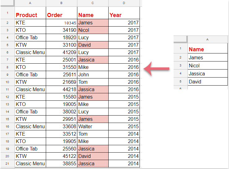
Định dạng có điều kiện để đánh dấu các ô dựa trên danh sách từ một trang tính khác trong Google Trang tính

Vui lòng thực hiện theo các bước sau để hoàn thành công việc này:
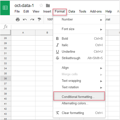
1. Nhấp chuột Định dạng > Định dạng có điều kiện, xem ảnh chụp màn hình:
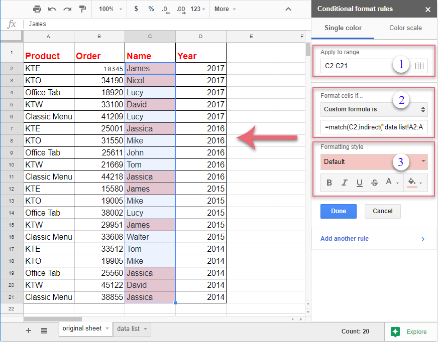
2. Trong Quy tắc định dạng có điều kiện , vui lòng thực hiện các thao tác sau:
(1.) Nhấp vào  để chọn dữ liệu cột mà bạn muốn đánh dấu;
(2.) Trong Định dạng ô nếu danh sách thả xuống, vui lòng chọn Công thức tuỳ chỉnh là và sau đó nhập công thức này: = match (C2, gián tiếp ("danh sách dữ liệu! A2: A"), 0) vào hộp văn bản;
(3.) Sau đó chọn một định dạng từ Kiểu định dạng như bạn cần.
Chú thích: Trong công thức trên: C2 là ô đầu tiên của dữ liệu cột mà bạn muốn đánh dấu và danh sách dữ liệu! A2: A là tên trang tính và phạm vi ô danh sách chứa tiêu chí bạn muốn đánh dấu các ô dựa trên.
3. Và tất cả các ô phù hợp dựa trên các ô danh sách đã được đánh dấu cùng một lúc, sau đó bạn nên nhấp vào Thực hiện nút để đóng Quy tắc định dạng có điều kiện ngăn như bạn cần.
Công cụ năng suất văn phòng tốt nhất
Nâng cao kỹ năng Excel của bạn với Kutools for Excel và trải nghiệm hiệu quả hơn bao giờ hết. Kutools for Excel cung cấp hơn 300 tính năng nâng cao để tăng năng suất và tiết kiệm thời gian. Bấm vào đây để có được tính năng bạn cần nhất...
")
Tab Office mang lại giao diện Tab cho Office và giúp công việc của bạn trở nên dễ dàng hơn nhiều
- Cho phép chỉnh sửa và đọc theo thẻ trong Word, Excel, PowerPoint, Publisher, Access, Visio và Project.
- Mở và tạo nhiều tài liệu trong các tab mới của cùng một cửa sổ, thay vì trong các cửa sổ mới.
- Tăng 50% năng suất của bạn và giảm hàng trăm cú nhấp chuột cho bạn mỗi ngày!
")